Conquering the Maze of Machine Learning with Q-Learning: The Off-Policy Temporal Difference Control Algorithm 🤖

📌 Let’s explore the topic in depth and see what insights we can uncover.

⚡ “Imagine a world where machines remember their past mistakes and use them to make better decisions in the future. Welcome to the realm of Q-Learning, where algorithms have the power of retrospection!”

Hello, future Machine Learning wizards! 👋 Today, we’re diving deep into the fascinating world of reinforcement learning, specifically focusing on one of its core techniques: Q-Learning. This powerful algorithm has helped machines navigate through virtual mazes, play video games, and even trade stocks. Sounds exciting, right? 🕹️ So, buckle up as we demystify the off-policy temporal difference control algorithm that has shaped the landscape of Machine Learning. Whether you’re a beginner dabbling in the field or a seasoned pro looking to brush up on the basics, this post is for you. By the end, you’ll have a solid understanding of Q-Learning, its inner workings, and how to implement it in your projects.

🔍 What is Q-Learning?

"Unleashing Power with Q-Learning Algorithm"

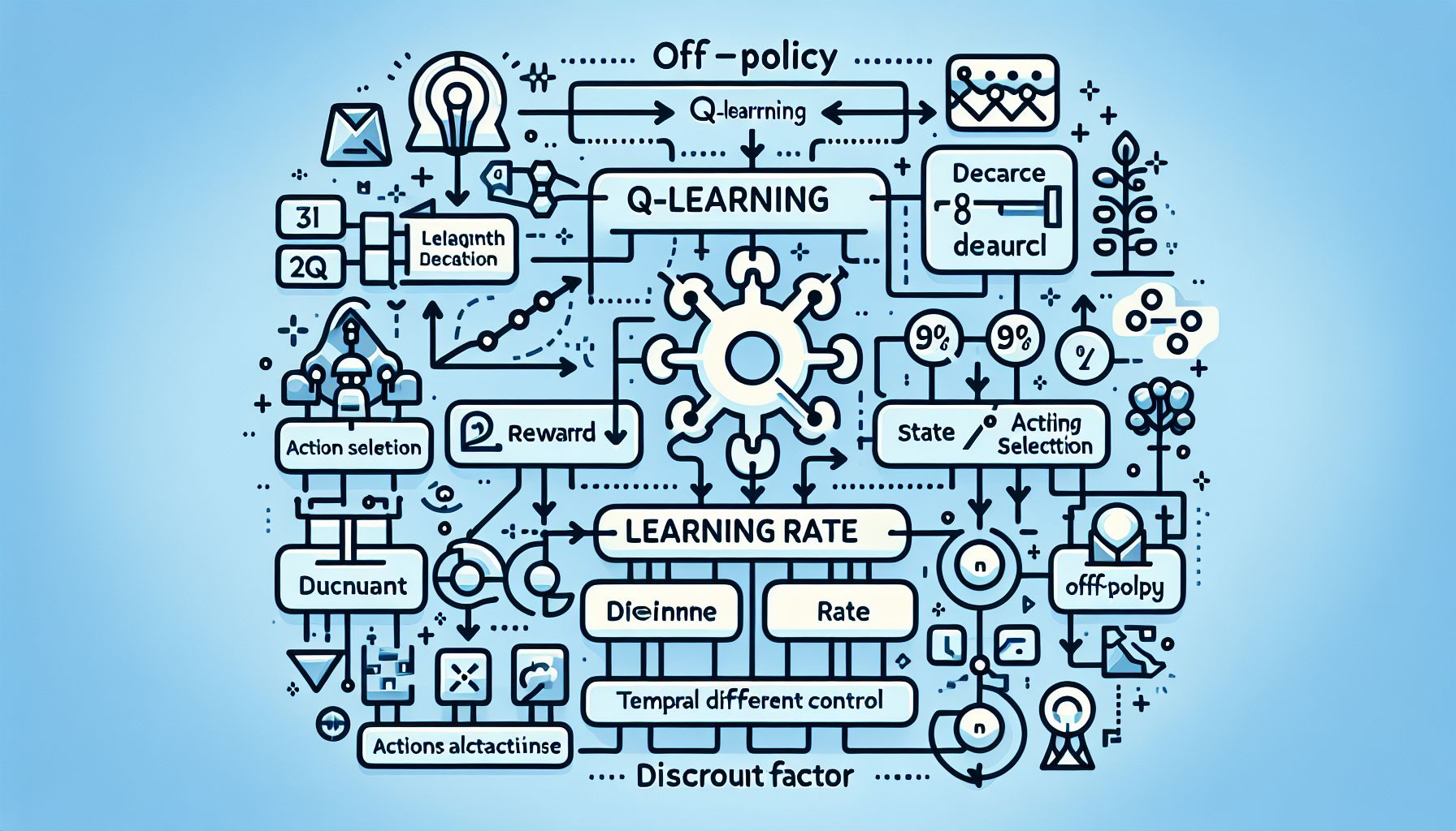
First things first, let’s tackle the basics. Q-🧠 Think of Learning as a value-based Reinforcement Learning algorithm that is used to find the optimal action-selection policy for a given Markov Decision Process (MDP). In simple words, it helps an agent (our machine learner) to choose the best action in a particular state based on its past experiences. 🗺️ Unlike other Reinforcement Learning algorithms, Q-Learning is an off-policy learner. This means it learns the value of the optimal policy irrespective of the policy being followed, providing a flexibility that makes it quite special. The ‘Q’ in Q-Learning stands for ‘quality’. It represents the quality of a particular action in a particular state. The higher the Q-value, the better the action.

🧮 The Math Behind Q-Learning

Don’t worry, we’re not about to dive into a sea of complex equations. The math behind Q-Learning is actually quite straightforward. At the heart of the algorithm is the Q-Learning update rule, also known as the Bellman equation: Q(s,a) ← Q(s,a) + α * [R(s,a) + γ * max Q(s',a') – Q(s,a)]

Let’s break it down:

Q(s,a): the current Q-value, representing the quality of performing action a in state s.
α: the learning rate (between 0 and 1). It determines how much new information overrides old information.
R(s,a): the immediate reward received after performing action a in state s.
γ: the discount factor (between 0 and 1). It determines the importance of future rewards.
max Q(s',a'): the estimate of optimal future value, achieved by performing the best action at the next state s'. This equation is at the core of the agent’s learning process. Through repeated application of this update rule, the Q-values tend towards their optimal values, allowing the agent to select the best actions.

📈 Implementing Q-Learning: A Step-by-Step Guide

Now that we’ve covered the theory, let’s dive into a practical example. Let’s imagine that our agent is a mouse 🐭 trying to find cheese 🧀 in a maze.

Initialize Q-Values

Start by initializing the Q-value table. This table will guide the mouse’s decisions. Initially, it’s filled with zeros, indicating that the mouse doesn’t know which way to go.

Choose an Action

The mouse needs to decide which direction to move in. It can either explore the maze by choosing a random direction or exploit its current knowledge by choosing the direction with the highest Q-value.

Perform the Action and Update Q-Value

The mouse moves in the chosen direction. It then uses the Q-Learning update rule to update the Q-value of the performed action.

Repeat

The mouse repeats steps 2 and 3 until it finds the cheese or a maximum number of moves is reached. This constitutes one episode.

Multiple Episodes

The entire process is repeated over multiple episodes, gradually improving the Q-value table, and hence the mouse’s policy.

Here’s some pseudo-code to help visualize the process:

### Initialize Q(s, a) arbitrarily
### Repeat (for each episode):
### Initialize s
### Repeat (for each step of episode):
### Choose a from s using policy derived from Q (e.g., ε-greedy)
### Take action a, observe r, s'
### Update Q(s, a) using the Q-Learning update rule
        s ← s'
    until s is terminal

🎯 Applications of Q-Learning

From video games to robotics, Q-Learning has a broad range of applications. It’s been used in:

Game AI: Q-Learning has been successfully used to train AI to play games like Pac-Man and Chess.
Robot Navigation: Robots can use Q-Learning to learn how to navigate through complex environments.
Resource Management: Q-Learning can be used to optimize resource usage in computer systems.
Stock Trading: Some high-frequency trading algorithms use Q-Learning to decide when to buy or sell stocks.

🧭 Conclusion

Q-Learning, the off-policy temporal difference control algorithm, is a powerful tool in the Machine Learning toolbox. Despite its simplicity, it provides the foundation for more advanced techniques and has proven to be effective in a wide range of applications. As with any Machine Learning technique, mastering Q-Learning requires both understanding the theory and getting your hands dirty with practical implementation. So, don’t stop here. Implement a Q-Learning agent and watch it navigate through the maze of your choice. Remember, the best way to learn is by doing. 🚀

Happy learning, and may your Q-values always converge!

🚀 Curious about the future? Stick around for more discoveries ahead!