📌 Let’s explore the topic in depth and see what insights we can uncover.
⚡ “Ever puzzled how a bird remembers the exact location of thousands of seeds it’s stored? Welcome to the remarkable world of Eligibility Traces and the TD(λ) Learning Algorithm!”
Imagine for a moment that you’re in a maze, and you’re trying to find the quickest path to the exit. You don’t have a map or a guide. All you can do is roam around, get lost, and learn from your mistakes. 🔍 Interestingly, precisely how reinforcement learning algorithms work. They learn by trial and error, gradually improving their performance until they find the optimal solution. One such algorithm is the Temporal Difference Learning (TD Learning) algorithm. It’s a model-free reinforcement learning technique that is particularly useful in predicting the outcome of an event based on past experiences. However, in its standard form, TD learning has a limitation – it doesn’t consider the importance of the sequence of states leading to the current state. 🔍 Interestingly, where Eligibility Traces and the TD(λ) Learning Algorithm come in. In this blog post, we will dive deep into the world of Eligibility Traces and the TD(λ) Learning Algorithm. From understanding their definitions to exploring their applications, we’ll uncover the magic behind these powerful tools in reinforcement learning. So, buckle up and let’s get started! 🚀
📚 Understanding Eligibility Traces

"Unraveling the Complexity of TD(λ) Learning Algorithm."
Before we dive into the nitty-gritty of the TD(λ) learning algorithm, it’s essential to understand what eligibility traces are and how they work.
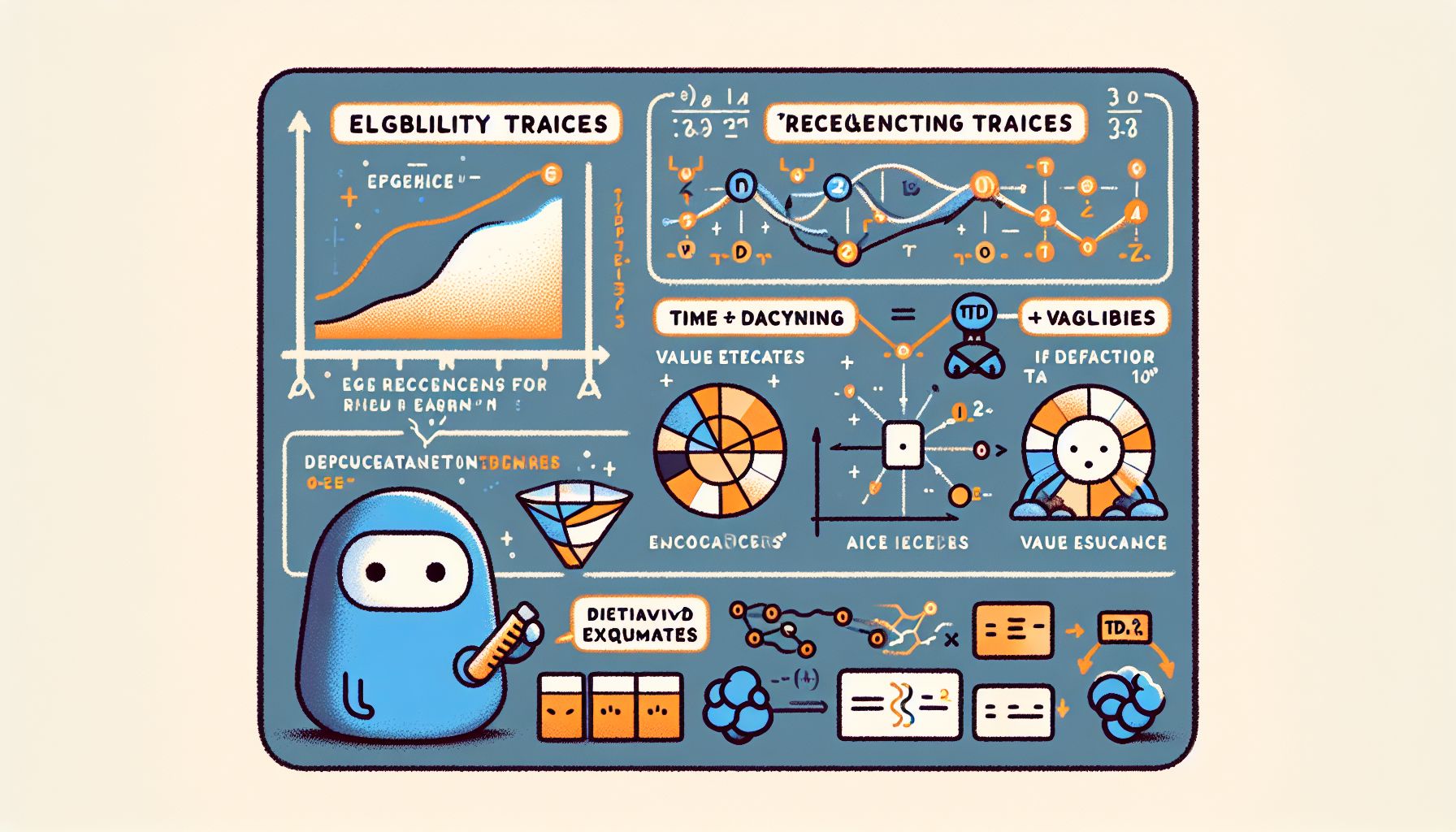
An Eligibility 🧠 Think of Trace as a memory tool used in reinforcement learning algorithms, allowing the agent to remember its past states and actions. Think of it as a trail of breadcrumbs 🍞 left by the algorithm to remember its previous steps.
The idea behind an eligibility trace is simple. When an agent is in a state ‘s’ and takes an action ‘a’, it leaves behind a trace. The trace’s intensity depends on the current reward and how recently the state-action pair has occurred. Over time, the trace fades away, much like the memory of a dream after waking up.
In mathematical terms, the eligibility trace for a state-action pair (s,a) is denoted as E(s,a) and is updated as follows:
E(s,a) = γλE(s,a) + 1
Here, γ is the discount factor, λ is the trace-decay parameter, and the ‘+1’ signifies that the current state-action pair has occurred.
🧠 The TD(λ) Learning Algorithm
Now that we’ve got a handle on eligibility traces, let’s dive into the TD(λ) learning algorithm.
The Temporal Difference Learning algorithm, or TD Learning for short, is a reinforcement learning algorithm that learns by predicting future rewards based on current states and actions. However, standard TD Learning considers only the immediate reward and doesn’t take into account the sequence of events leading up to the current state.
🔍 Interestingly, where the TD(λ) learning algorithm comes in. The λ in TD(λ) stands for the trace-decay parameter we saw earlier in the eligibility traces. The TD(λ) algorithm uses eligibility traces to help the agent remember its past states and actions, hence considering the sequence of events leading up to the current state.
The TD(λ) algorithm updates the value function (V) for each state-action pair (s,a) using the following formula:
V(s) = V(s) + αδE(s,a)
Here, α is the learning rate, δ is the Temporal Difference error, and E(s,a) is the eligibility trace.
💡 Advantages of TD(λ) and Eligibility Traces
By now, you should have a good understanding of how the TD(λ) algorithm and eligibility traces work. But why should you consider using them? Let’s look at the advantages they offer.
Better Credit Assignment
By considering the sequence of states leading up to the current state, the TD(λ) algorithm assigns credit more accurately for actions leading to a reward.
Efficient Learning
The TD(λ) algorithm can learn more efficiently than standard TD Learning, as it uses past experiences to influence future decisions.
Temporal Abstraction
The TD(λ) algorithm provides a way to handle temporal abstraction, where actions have consequences that may not be immediate.
Adaptability
The trace-decay parameter λ can be adjusted to fine-tune the algorithm’s performance. A larger λ means more weight is given to past states, while a smaller λ gives more weight to recent states.
🧩 Practical Applications of TD(λ)
The TD(λ) algorithm and eligibility traces are not just theoretical concepts. They have practical applications in various fields. Here are a few examples:
Game Playing
TD(λ) has been used in game-playing algorithms, like the famous TD-Gammon, a computer program that learned to play backgammon and even beat human world champions.
Robotics
In robotics, TD(λ) can be used for problems like navigation, where the robot needs to find the quickest way to a goal.
Recommendation Systems
TD(λ) can be applied to recommendation systems to predict user preferences based on past behavior.
🧭 Conclusion
From a humble breadcrumb trail in a complex maze to powerful algorithms that can beat world champions at board games, the journey of Eligibility Traces and the TD(λ) Learning Algorithm is quite fascinating. They offer a unique approach to reinforcement learning, giving consideration to the sequence of events leading up to a decision, thus enabling more accurate and efficient learning. With their practical applications in fields like game playing, robotics, and recommendation systems, these tools are truly magic wands in the realm of reinforcement learning. So next time you find yourself lost in a maze, remember the TD(λ) algorithm and its trail of breadcrumbs. Who knows, it might just help you find your way!
🤖 Stay tuned as we decode the future of innovation!
